
2 posts tagged with "sql"

View All Tags

· 13 min read

The purpose of this blog is to show off the ease of importing from external data into Zef and using a proxy view to expose Zef to 3rd-party packages. It is also a diary of how the development of these features worked, allowing me to polish them as we go!

There are many reasons you could want to expose a Zef graph using networkX:

  • You have existing code that uses the networkX framework
  • You want to use a 3rd party library that can accept a networkX graph, for example a plotting library like plotly.
  • You want to use a graph analysis algorithm that isn't yet available in Zef.

The outline of this process is:

  1. Get some external data
  2. Import it into a Zef graph
  3. Expose the data using a "proxy"
  4. Do the analysis
  5. Spit out some pretty visualisations

In this post, I will focus only on the highlighted points 1 and 2, i.e. getting your data into a Zef graph.

1. Get some external data

We'll use the Northwind dataset as an example, which describes sales and orders for a company. This is available from here https://code.google.com/archive/p/northwindextended/downloads. To convert this to CSV files, I wrote a little script available export.py, which creates a temporary SQLite DB to export each table as its own CSV file. If you'd like to follow along as home, to save you the bother I've made these CSV exports available northwind.zip.

After running this script, we find there are 14 CSV files in this dataset. I'll use products.csv to demonstrate some of the features below and its first few rows look like:

ProductIDProductNameSupplierIDCategoryIDQuantityPerUnitUnitPriceUnitsInStockUnitsOnOrderReorderLevelDiscontinued
1Chai8110 boxes x 30 bags18390101
2Chang1124 - 12 oz bottles191740251
3Aniseed Syrup1212 - 550 ml bottles101370250
..............................

So long as the CSV files can be imported using the pandas python module, then we are able to import these into a Zef graph.

2. Import into Zef

If you have seen the "Import from CSV" how-to in our docs, you might first think to jump straight to the Zef pandas_to_gd op to import it. However, the CSV files in this dataset are in a representation that is best suited for SQL, with columns representing both fields AND relationships between different entities.

Instead, we need to provide a declaration for the set of tables that the CSV files represent, which all together produce the right graph structure. For example, we should be able to specify the purpose of each column in the products.csv table to be something like:

ProductIDProductNameSupplierIDCategoryIDUnitPrice...
PurposeIDFieldEntityEntityField...
ETET.ProductET.SupplierET.Category...
RTRT.IDRT.ProductNameRT.SuppliedByRT.InCategoryRT.UnitPrice...
Data typeIntStringIntIntQuantityFloat.dollars...

The above is just a layout for me to organise my thoughts on what each column should do. I could have instead said the above in sentences:

  • The ProductID column should represent the ID of the ET.Product entities which this table defines in each row. The IDs will be stored on the Zef graph using RT.ID relations.
  • The ProductName column gives fields for each row, which will have a relation type of RT.ProductName and be a string.
  • The SupplierID column is a different entity of type ET.Supplier, uniquely identified by the integer in this column. It is linked to the ET.Product via a RT.SuppliedBy relation.
  • ...

We will need to introduce a couple of more "purposes" in a moment, but otherwise this has nearly covered all of the main uses of the dataset.

Writing this all out by hand is tedious, so I wrote up a quick parser in Zef to produce the initial layout for you and then allow you to edit it. I made the following by running:!!!

from zef.experimental import sql_import

decl = sql_import.guess_csvs("products.csv")

decl | write_file["guess.yaml"] | run

then editing the file guess.yaml a little bit:

default_ID: ID
definitions:
- tag: products
data_source:
filename: products.csv
type: csv
kind: entity
ID_col: ProductID

cols:
- name: ProductID
purpose: id
RT: ID
data_type: Int

- name: ProductName
purpose: field
RT: ProductName
data_type: String

- name: SupplierID
purpose: entity
ET: Supplier
RT: SuppliedBy
data_type: Int

I then wrote up a function import_actions which will take this declaration of how to map the CSV data to the graph and do the busy-work to product a graph. Here is how to run that:

decl = "edited.yaml" | load_file | run | get["content"] | collect
g = Graph()
actions = sql_import.import_actions(decl)
actions | transact[g] | run

The import_actions function will use the information in decl to find the files from which to read the raw data.

While the above works okay on the products.csv table, I needed to include two more things to allow the import of all CSV files simulataneously: a way to tag a table as a "entity" or "relation" style and a source/target purpose.

Interlude into GUI land

Editing the yaml file by hand is clunky. However, it does have the benefit of being easy to a) read as plain text, and b) save the declaration of the import without custom data structures.

To get rid of the clunkiness, and also indulge myself to explore a new package, I decided to write a little UI using pyimgui to better edit the file. Try it out on my sample sql_import.yaml with:!!!

python -m zef.experimental.sql_ui.wizard sql_import.yaml

You should see something like:

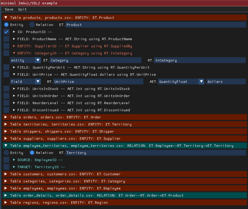
The UI is in its early stages so might not work fully. It also requires installing the pyimgui module with sdl support (i.e. pip3 install pyimgui[sdl2] or the like). Weirdly this seems to have problems with python version 3.10 on macos... we will be looking into this.

To read more about using this GUI, check out our docs page on Multiple interlinked CSVs

"relation" kinds of tables

If there is a one-to-many or many-to-many relationship between two objects in a SQL database, then there are various ways to represent this. In the Northwind example, the "Order Details" table demonstrates this, as it allows each Order to contain multiple different products (the one-to-many relation), with particular (order,product)-specific prices, quantities and discounts.

OrderIDProductIDUnitPriceQuantityDiscount
102481114120.0
10248429.8100.0
102487234.850.0
102491418.690.0
...............

Hence we can think of this table as not being entity-centric but rather relation-centric. Any fields (e.g. the UnitPrice column) is information that should be attached to the relation between the order and the product. As Zef graphs we always have directed relations, so we need to also specify a "source" and "target" column:

OrderIDProductIDUnitPriceQuantityDiscount
PurposeSourceTargetFieldFieldField
ETET.OrderET.Product
RTRT.UnitPriceRT.QuantityRT.Discount
Data typeIntIntQuantityFloat.dollarsIntFloat

The import!

My full processing of the CSV files is shown below. My edits to the sql_import.yaml file are available here: sql_import.yaml.

from zef import *
from zef.ops import *
from zef.experimental import sql_import

decl = sql_import.guess_csvs("*.csv")
decl | write_file["sql_import.yaml"] | run

# ... edit sql_import.yaml externally...

decl = "sql_import.yaml" | load_file | run | get["content"] | collect
g = Graph()
actions = sql_import.import_actions(decl)
actions | transact[g] | run

After this import, the graph looks like:

>>> yo(g)

<...snip...>
^^^^^^^^^^^^^^^^^^^^^^^^^^^^^^^^^^^^^^^^^ Atomic Entities ^^^^^^^^^^^^^^^^^^^^^^^^^^^^^^^^^^^^^^^
[6007 total, 6007 alive] AET.String
[2985 total, 2985 alive] AET.Float
[2527 total, 2527 alive] AET.Int
[2232 total, 2232 alive] AET.QuantityFloat.dollars
[2469 total, 2469 alive] AET.Time

^^^^^^^^^^^^^^^^^^^^^^^^^^^^^^^^^^^^^^^^^^^^ Entities ^^^^^^^^^^^^^^^^^^^^^^^^^^^^^^^^^^^^^^^^^^^
[1660 total, 1660 alive] ET.Order
[154 total, 154 alive] ET.Product
[12 total, 12 alive] ET.Employee
[93 total, 93 alive] ET.Customer
[53 total, 53 alive] ET.Territory
[4 total, 4 alive] ET.Region
[3 total, 3 alive] ET.Shipper
[29 total, 29 alive] ET.Supplier
[8 total, 8 alive] ET.Category

^^^^^^^^^^^^^^^^^^^^^^^^^^^^^^^^^^^^^^^^^^^ Relations ^^^^^^^^^^^^^^^^^^^^^^^^^^^^^^^^^^^^^^^^^^
[4 total, 4 alive] RT.RegionDescription
[4 total, 4 alive] (ET.Region, RT.RegionDescription, AET.String)
[2155 total, 2155 alive] RT.Order
[2155 total, 2155 alive] (ET.Order, RT.Order, ET.Product)
[9 total, 9 alive] RT.ReportsTo
[9 total, 9 alive] (ET.Employee, RT.ReportsTo, ET.Employee)
<...snip...>

If you don't want to do the import yourself, you can also look at the graph that I created at the tag zef/blog/northwind, that is, you can access it via:

g = Graph("zef/blog/northwind")

Final comments

As always, answering a simple question has opened up many more questions which I can't help myself but discuss below...

One final purpose: "field_on"

There's another addition that's needed to import many production SQL tables: a way to handle databases with optimised tables.

While we do not need this kind of purpose for the Northwind dataset, it is useful to mention it to "complete the story". The above example of the "Order Details" table which produced pure relations (and not entities) is because the Northwind dataset is in "first normal form".

A "denormalised" dataset could also be used for performance reasons. For example, obtaining all of the products ordered by a particular customer would require an SQL JOIN query to obtain:

SELECT DISTINCT(order_details.ProductID)
FROM order_details INNER JOIN orders
ON order_details.OrderID = orders.OrderID
WHERE orders.CustomerID = "VINET";

Instead, the join of orders and order_details could itself be stored as a table (or view) in the SQL database:

OrderIDCustomerIDOrderDate...ProductIDQuantity...
10248VINET1996-07-04...1112...
10248VINET1996-07-04...4210...
10248VINET1996-07-04...725...
10249TOMSP1996-07-05...149...
10249TOMSP1996-07-05...5140...
.....................

The concept of avoiding joins is rather weird when coming from a graph perspective, as the equivalent of joins are trivial on a graph. However, you may not have any choice in the data you want to import. In this case, we can mark those columns as belonging to the relation between the order and product using "field_on":

OrderIDCustomerIDOrderDateProductIDQuantity
PurposeIDEntityFieldEntityfield_on
ETET.OrderET.CustomerProduct
RTIDCustomerRT.OrderDateRT.ProductRT.Quantity
TargetProductID
Data typeIntIntTimeIntInt

Here the "Quantity" column cannot be set as a field as it would have multiple values for the same ET.Order. So instead we designate that it should be attached to the "target" column ProductID. This means we could write a Zef query for the total quantity of an order as:

z_order > L[RT.Product] >> RT.Quantity | value | add | collect

Batteries-included?

The imported tables still duplicate a lot of information. For example, each of the ET.Order, ET.Supplier, ET.Customer, ET.Employee have a RT.Region which is a scalar string. This is not very connected, as it would be better to have these RT.Regions point at a ET.Region. That way, we could ask for all suppliers in the same region as a customer without doing string matching.

I was tempted to add this in as another purpose, something like entity_from_matching_field. But this would have degenerated into providing an arbitrary language to describe the endless possible databases out there. Instead, we can post-process the imported Zef graph, which gives us access to the entire Zef ops capabilities.

You might be worried about exposing the gorey details of the import process and only the post-processed data. This is easy, if we export only g | now to a new graph after performing the post-processing.

A comment on speed

If you run the commands in this blog post on a large dataset, then you are going to be waiting several minutes for the import. Even as part of writing this post up, and using the Northwind dataset which is relatively small, I found I had to optimise some aspects of the GraphDelta implementation.

This is largely due to the current pure-python implementation of the evaluation engine for ZefOps. In the future this will be implemented in C++ along with the core of the GraphDelta code.

Import directly from SQL

To be honest this blog post is a little crude, using CSV files which lack type information rather than the SQL source directly. The information available in the SQL schema can also assist automatic detection of connected entities and whether a table represents a single entity or many-to-many relations.

The benefit of handling CSV files is it allows us to accomplish almost all kinds of imports, so long as we provide enough additional information. If we supported only SQL, then this would limit the flexibility.

The other reason that the SQL schema is not used directly, is that it's a fair bit more work to support a SQL connection or export. But our intent is to extend these tools and make imports as close to one-click as possible!

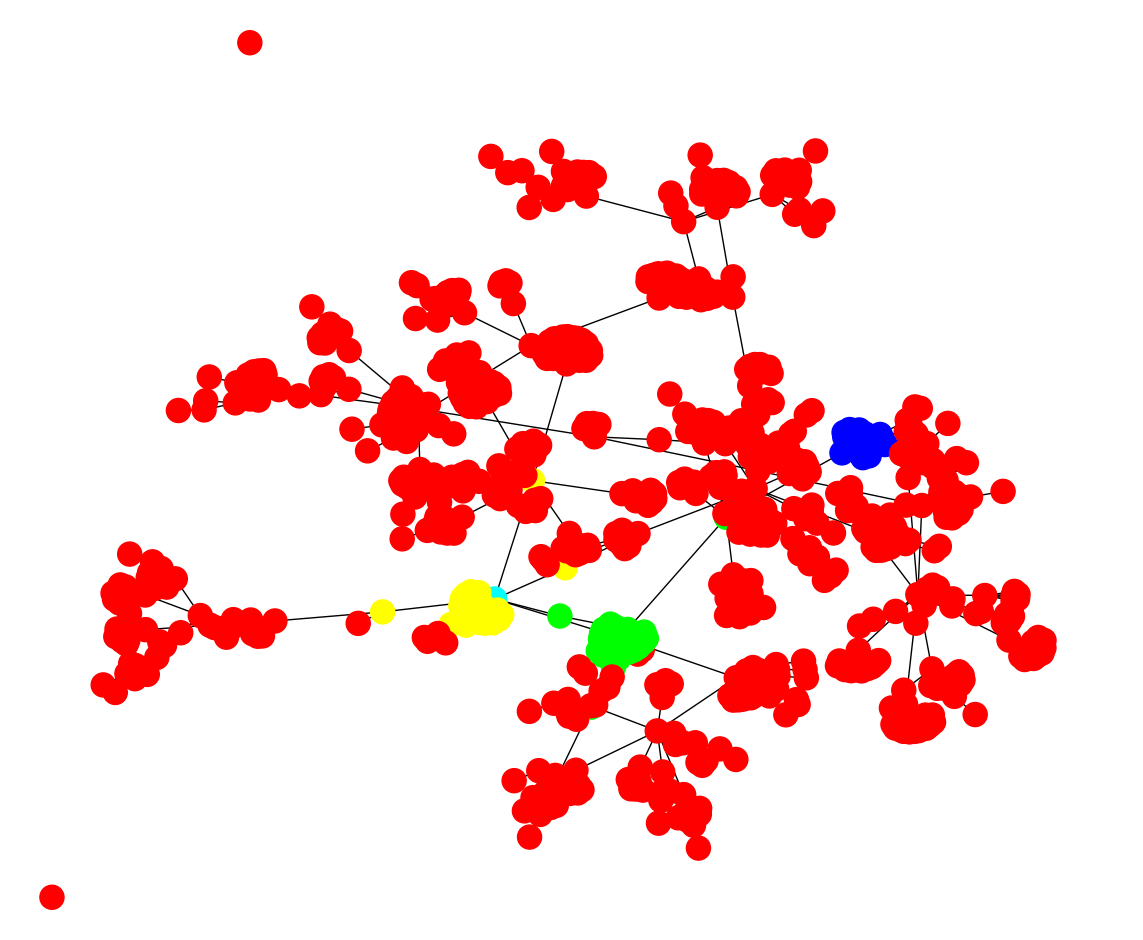
Analysis using external tools

I'll leave this for the next blog post! But as a sneak preview...

Wrap up

If you'd like to find out more about Zef and ZefHub (and get early access), get us out at zefhub.io.

· 13 min read

One major motivating factor that is often associated with relational databases is the ability to interact and query the data declaratively. Instead of telling the DB exactly how to traverse and gather the data, just give a bunch of clauses that have to be true and let the DB figure out how to resolve the query most effectively.

q1 = Query([
Z['p1'] | is_a[ET.Person],
Z['p1'] >> RT.FirstName | value | equals['Roger'],
])
SELECT * from Persons WHERE FirstName="Roger"
  • everything in SQL is a table: entities are defined as rows of attributes. In Zef an Entity can "just be". It may have have attributes expressed as relations to values or atomic entities.
  • variables from predicate logic are the equivalent of columns / column names in SQL.
q2 = Query([
Z['x1'] | is_a[VT.Int],
Z['x1'] | less_than[5],
Z['x1'] | greater_than[0],
])
  • Z['x1'] is a variable in the sense of predicate logic. In other fields they are sometimes also referred to as "unbound constants".
  • We have to wrap it with Z, since using x1 by itself on the spot would not be valid Python syntax
  • We could declare all variables used beforehand if the Z bothers us: x1 = Z['x1']
  • each line is a predicate function: given a potential solution, it can be evaluated to true or false
  • these predicate functions are often called "clauses" in mathematical logic - don't be frightened by the name
  • each line can contain one or more variables: predicates can thus also express constraints between variables.
  • the solution to a given query / list of constraints MUST fulfill each individual predicate. I.e. it can just be seen as one big predicate function obtained by combining all of them via an And.
  • This combined predicate function is a function of all variables occurring in the query.
  • We can also see each individual predicate function as a function off all variables in the query if we want a more formal justification for combining them with an And (the logical operators can only combine predicates with the same function signature)

Let's take the previous query up a notch:

q3 = Query([
Z['p1'] | is_a[ET.Person],
Z['p2'] | is_a[ET.Person],
Z['p1'] >> RT.FirstName | value | length | equals[
Z['p2'] >> RT.FirstName | value | length
],
])

Just to put it in normal words: "please return me all pairs of persons whose first names are of the same length." A result of this query would be a (possbily very long) list of dicts, each containing two people [{'p1': z_jack, 'p2': z_john}, ... where z_john and z_jack are both ZefRefs and point to persons with those names respectively.

But this is not what we want to get at. The crucial part we want to demonstrate here is that to express queries of this type succinctly, we need the ability to use ZefOps inside predicate functions. It is crucial that these are not lazy values that can be evaluated to a fixed value beforehand, but they involve variables themselves. These only become equivalent to lazy values within the context of a potential solution.

So what is the problem? Before we were using greater_than[0], i.e. a value inside the combinator, whereas now we are using a clause. Also: clauses can be understood as Zef lambda functions (as we discuss elsewhere). And Zef lambda functions are values themselves within Zef: value semantics is one of the foundational principles that we cannot give up. So now we are using greater_than with two different values, but in quite different ways. This is a problem: what is the nature of the thing we pass into equals? Should the second case only return true if the argument piped in is the very Zef Lambda function inside? This seems to be the case at first glance, if we want strict and general value semantics. But there is a way out and one also encounters it in different contexts. It is actually an approach that dates all the way back to Alonso Church, who came up with lambda calculus, which you may have heard of. The way out of our dilemma is just to put on our Church glasses: in lambda calculus everything is a function. Even an integer like 42 can be seen as a function: it is simply the function that returns 42 whatever argument you give it. What are the arguments here and why are they not listed? Because it would be too tedious. As we saw, a query can be seen as one big lambda function itself that is just the combination of all listed clauses combined with And. The variables are implicit and are all the variables that occur in the query. This allows us to keep our short syntax in terms of values above, e.g. use greater_than[0] with it having exactly the simpler meaning we associated with it before. The occasional user of Zef does not even need to be aware of all this abstract stuff and lambda calculus.

So what does this mean concretely? How can we construct a semantically consistent system out of this? There is a very narrow path out of this mess. We can simply be guided by the logical constraint and the goal of a succinct, not overly technical syntax. We do not want to require everyone to have to syntactically wrap their values in a lambda function.

Let's go through the requirements:

  1. A value 42 is distinct from the Zef lamba function func[42] that always returns 42.
  2. values inserted into logic operators must be interpreted as Zef Lambdas
  3. We don't want to write the func[...] wrapper everywhere
  4. All of this is not specific to equals, but applies to all logic operators (unary, binary, all arities)

Hence, anything injected into a [...] of a logic operator will be understood to be wrapped by a func[...] at the point of evaluation. This may sound horribly complicated at first, but keep your pitch fork down for a moment. What we're after is that the resulting syntax is easy to use and consistent. The expression 42 | equals[42] will continue to evaluate to true, since the two associated Zef lambdas (which are values themselves) are considered to be equal.

Side note: note that lambdas in Python do NOT follow value semantics for functions in this sense:

my_answer_to_everything   = (lambda : 42) 
your_answer_to_everything = (lambda : 42)
should_we_start_a_flame_war: bool = my_answer_to_everything != your_answer_to_everything

# OMG Python, you're worse than social media!
print(should_we_start_a_flame_war) # True

But now we notice that this also allows us to throw in other expressions and operators that will be interpreted accordingly: both cases that we started off with, e.g. using greater_than[0] and but also greater_than[ Z['x1']>> RT.Age | value ] would work. At the point of evaluations, the latter internal argument is translated into func[ Z['x1']>> RT.Age | value ] which by itself is a valid Zef lambda function that could be used in a different context as well.

The one thing we are not allowed to do is wrap the expression in an additional func[] layer and expect the same behavior. E.g. equals[ func[Z['x1']>> RT.Age | value] ] would check whether the incoming value is equal to that lambda function, i.e. at the point of evaluation func[ func[Z['x1']>> RT.Age | value] ] is the Zef lambda function that always returns the internal lambda function (a value itself), not matter what arguments are passed in.

So what does this mean, you may ask? The take away message for Zef lambda syntax is that multiple layers of func[...] do not automatically collapse to a single wrapping func[...] layer. They are different things.

What about using Python lambdas in piped expressions? since 42 | (lambda x: x+1) cannot be intercepted by Zef in any way without doing unspeakably horrible things, you will have to wrap raw python functions and lambdas in one layer of func[...]:

42 | func[lambda x: x+1] | collect

works and is the way you have to do it. The same goes for normal python functions. But as soon as you have a Zef function, wrapping it in a func[...] will cause an additional layer of wrapping, since that Zef function is itself already a Zef value. This is the gotcha to watch out for!

SQL & Zef

Declarativeness is in the Eye of the Beholder

Knowing ones own type

How does an entity / object know what it is?

Classes / Structs

This depends on the programming language. In dynamic languages like Python, this is stored as explicit meta-information as a pointer on each object pointing at the parent type object. In compiled languages like C++, this information may not even be stored explicitly at runtime: only the struct's/object's contained attributes are stored at the objects location in memory. The information about which type it is compiled away in the simple case (this may be different for typed unions, e.g. std::variant and other more advanced structures).

JSON / Python Dicts

This is either implicit from the context in which the dictionary is stored. Often the associated entity's type may also be explicitly stored as a value under a "type" key.

Relational Databases / Spreadsheets

Which table it is contained in: the table name can often be seen as the equivalent to the object's type. Each row in the table can be seen as an object/entity expressed in terms of its attributes / fields (columns).

Document Database

These are often organized in terms of collections. Just like we know that the real world entity described by a row in a table knows what it is from the table's name, a document in a collection is specified by the name of the collection. In some cases users may find it more convenient to directly dump json into the database.

Zef Graphs

Each Relation / Entity / Atomic Entity (RAE) has its type stored explicitly in its blob on the graph. In contrast to objects, RAEs have no internal structure whatsoever. Rather than choosing to model the world in terms of a hierarchical taxonomy, all information is represented associatively in terms of relations.

History of Zef: Evolving from Property Graphs

"Perfection is achieved, not when there is nothing more to add, but when there is nothing left to take away." — Antoine de Saint-Exupéry

The Zef data model may seem somewhat strange at first when coming from the world of objects, tables or property graphs. In this post we want to give a brief overview of how we arrived at this data structure. Maybe we can even convince you that it is a simpler data structure than many of the better known alternatives.

1) model our domain in terms of C++ structs / Python objects 2) move to using plain old dictionaries, all the serialization and de-serialization code was getting too much 3) having to choose a hierarchy does not play well with modelling a complex domain where requirements often change. We often thought we got the domain modeling wrong, but that was missing the true underlying reason: the real world domain model was that of a graph and different parts of our system require querying the data from different directions. Choosing any tree-based hierarchical data structure has a structural mismatch with the true domain model. We moved on to use NetworkX. What a relief, working directly in terms of graphs is awesome! Why is this not the norm? 4) NetworkX is a bit slow. Even for Python standards. Also, we really want to work on top of graphs in our high performance simulations written in C++. 5) After exploring multiple options (iGraph, Boost Graph, various DBs), we didn't find any that had user friendliness in terms of the API we were looking for and the performance we required. How hard could it be to build a more performant version, but very much stripped down version of NetworkX in C++ and expose bindings to Python. This was actually easer than we thought and a basic version of "Arachne" was up and running after two to three weeks. The core data structure was a directed property graph: both the nodes and edges could contain attributes. For the application that we were running (MCTS-like simulations), Arachne achieved about a 10000x speedup over NetworkX, which somewhat surpassed our expectations. Cache locality and data oriented design for the win! 6) This design took us pretty far, but there were three problems appearing. A) working in the field of manufacturing, our domain models between customers differed and were often quite complicated. Also, they were often evolving over time as new requirements and features came up. We noticed the following pattern reappear every few weeks: an initially unimportant field of some entity started off its life as an internal attribute on a node or an edge. But at some later point, it became more important and modelling it as an internal attribute no longer seemed like the right choice. It should be a separate entity on the graph. All of this implied a graph schema change (yes, Arachne graphs had schemas) and a migration of the production data together with all the different code snippets that tied into that attribute. We also noticed that the opposite direction never occurred: something we had started modeling as a separate entity on the graph never became an internal attribute and caused us hours of repetitive, boring work.

With this pattern emerging, what would the end game of this iterative domain model revision war be? A domain model where every attribute will have become its own distinct entity on the graph? That sounds silly and too radical. But what would happen if we actually tried this? What is the defining difference between an objects attribute and a separate entity connected by a relation in any case? Doesn't this distinction introduce two different languages for querying individual fields of entities on a graph: one for traversing the graph and one for accessing internal attributes. Would it not be simpler if we had a single language only and everything would just be a graph traversal. There is no inner structure to RAE, there is no externally imposed hierarchy on our domain model.

There was one complication though: Since Arachne was a directed property graph, we stored attributes for some relations on the graph as well. It was by far not as common as attributes of an entity, but they were extremely useful in some cases (suppose you were to model an online store with certain items added to an order. One of the simplest ways to store the number/amount of a given item is as an attribute of the "ordered" relation itself). What would become of these edge attributes when we flatten everything out on the graph? According to our recipe of representing fields as relations to separate "values nodes" on the graph, we would have relations coming out of relations?! This would no longer be a graph. However, after a fair amount of back and forth, this is exactly what we decided to do. Zef Graphs are thus not simple graphs, but "meta-graphs" (we found this naming in this paper by Ben Goertzel). Note that these are different from hypergraphs, which can have edges which can connect more than two nodes.