· 9 min read

In this blog, we will see how we can use ZefOps to solve Advent of Code - Day 13!

We will see how ZefOps, compared to plain Python or Python with other libraries, allows us to write short, readable and composable code.

Before you start reading, get familiar with the problem we are solving today and even give it a shot here before digging in.
AOC

Problem Explanation ❓

After reading the problem statement, let's explain and simplify some points:

  • We can divide our input into 2 lists:

    • points (x,y)
    • fold instructions (axis, val)
  • Each fold instruction could only reduce or maintain the number of points, but never increase them.

  • 2 points overlapping become the same point, thus reducing the number of points.

With these points in my mind, let us attempt the solution to part 1!

Solution Breakdown 💡

Parsing the Input

We will use for this blog, the input I was given while solving the problem, that will differ from yours.

The first step of almost all of Advent of Code problems is to parse the input. This is usually a daunting problem to beginners, but with ZefOps it won't be.

As mentioned above let us manually divide our big input into 2 strings, str_points and str_folds.

from zef.ops import *       # don't forget to import ZefOps module from zef

str_points: str = """..."""
str_folds: str = """..."""

Parsing Points String

We start by parsing str_points using this simple ZefOp chain:

points =  str_points | split["\n"] | map[split[","] | map[int]] | collect                    

We can also stack the chain like this for better readability:

points = (
str_points
| split["\n"] # ["897,393", "...]
| map[split[","] | map[int]] # [[897,393], [...]
| collect
)

Let us look at the simplicity of the ZefOps in parsing the input from a single string to a list of points [x,y].

We first used split["\n"], as the name suggests to split the string into a list of individual strings on each line: ["897,393",...]

Then we used, map[split[","] | map[int]] to map each individual string onto the smaller ZefOp chain which splits the line on the character , and maps each resulting string onto an int: [[897,393], [...]

We see in this small example how composable ZefOps are. We are able to stack ZefOp chains inside ZefOp chains

Lastly, we collect to evaluate the lazy expression.

Oh you didn't know that ZefOps were lazy by nature! Well now you know. Computation will only happen on ZefOp chains once you call collect or run collect is a ZefOp used at the end of a Zef pipeline that makes it eager and returns a value. Without collect, the expression is just data.

Parsing Fold Instructions Strings

The second step is to similarly parse the fold instructions string str_folds.

foldings = (
str_folds
| split["\n"] # ["fold along y=6", ...]
| map[split[" "] | last | split["="]] # [["y", "6"], [...]
| map[lambda p: (int(p[0] == 'y'), int(p[1]))] # [(1, 6), ..]
| collect
)

As the first parsing, we split the long string over the new line character \n, then we map each string onto a small ZefOp chain split[" "] | last | split["="] which produces a list of lists of 2 strings ["axis", "value"].

We then map of these ["axis", "value"] lists, on a lambda expression that returns a tuple of (axis_encoded, value). The encoding of the axis will help us later. 0 for x and 1 for y.

Core logic

After parsing the input, it is time to write the logic of our algorithim to solve part 1!

Let me describe the algorithim flow in plain english and then we will see the equivilant Zef code.

  • For each point given a fixed axis 0 or 1 and a val to fold on,
    • If the point x or y, (0 or 1 i.e axis value) coordinate is larger than than val then return its new coordinate after the fold
    • Else just return the point itself, i.e it is on the side that won't be folded.
  • Cast the list of points on a set so that points that overlap become a single point, given that property of set.

The new coordinate of a point could be found using this simple algorithim.

Note either x or y will remain and the other will be mapped according to the equation:

  • If axis is x i.e 0 then:
    • point will be (val - (p[axis] - val), p[1])
  • Else
    • point will be (p[0], val - (p[axis] - val))

To understand how this work, make a simple matrix of points on a piece of paper and try to figure out how does a point's new location after a fold relates to its old position.

Putting this all together we can create a function fold that takes the list of points and fold_info and returns the new set of points after the fold has been performed.

def fold(points: set, fold_info: tuple) -> set:
axis, val = fold_info
new_coordinate = lambda p: ( (p[0], val - (p[axis] - val)) if axis == 1
else (val - (p[axis] - val), p[1]) )
dispatch = lambda p: new_coordinate(p) if p[axis] > val else tuple(p)
return set(
points
| map[dispatch]
| collect
)

As you can see from the code, we simply have 2 lambda functions to dispatch and return new coordinate and a simple ZefOp chain that maps each point onto the dispatch lambda function. The last step is to call set over the resulting list to remove duplicate points, points that now overlap.

Part 1

That is pretty much all the code we need to solve part 1. As stated in the problem statement, part 1 solution asks to find the number of points after the first fold instruction. So let's do that:

fold(points, foldings[0]) | length | collect 

We called fold with the starting lists of points and the first fold instruction, foldings[0]. As we said above, we will get back the set of points after the fold. All we gotta do is to just call length on that set, and that's the answer to part1!

Part 2

Part 2 is where it gets interesting as the problem statement makes it sound complicated but as a matter of fact, it is quite easy 😜

The idea is to run the points through the whole list of fold instructions in order and then somehow find a secret code 🕵🏻 encoded by the remaining points.

So this first step is to run our points through the whole list of fold instructions. But here is where it might be tricky, we run the points through one instruction and then with new set of points we run that over the next instruction. If that explanation wasn't a clue enough of what ZefOp to use, will we are going to use reduce. As the explanation suggests, with each fold instruction we reduce our points and pass that onto the next instruction. Until we have done all the instructions.

This looks as simple as:

foldings | reduce[fold][points]

After running reduce on the list of points, we need to now figure out the secret code.

So the idea, is to treat our remaining points as part of a Row x Col grid with Row being the highest y value in our list of points i.e number of rows, and respectively Col being the highest x value.

Now the fun part is to print this whole grid in our terminal, with 🟨🟨 for any (x,y) in our list of points and ⬜️⬜️ for any (x,y) that isn't in our points.

I know I know, this is all confusing but we are almost done! We put the logic above in a function output that takes the list of points!

def output(points):
for y in range((points | map[second] | max | collect) + 1):
for x in range((points | map[first] | max | collect) + 1):
if (x,y) in points: print("🟨🟨", end="")
else: print("⬜️⬜️", end="")
print("")

Let us put it all together now, where we run the result of the reduction on the output function like this:

foldings | reduce[fold][points] | run[output]

And the result is 🥁

Output

When I tell you I was shocked to see this, I am not lying. Probably one of the most exciting problems I got to do on Advent of Code!

Other Solutions 😓

For this portion of the blog, I scoured the internet for random Python solutions of AoC day 13 just to compare them with the ZefOp solution.

Bear in mind, beside the nice readability and composability of the ZefOp solution, if we remove the multiline chains, made for easier readability, the ZefOp solution stands at only 10 lines 😲!

Using Numpy, around 40 loc.

Using matplotlib around 45 loc.

Using plain python only around 50 loc.

Using plain python only around 70 loc.

Using Multiple Approaches around 35 loc.

These were some solutions that I randomly selected with no intention of offending their respective authors or critiquing their styles and solutions. The intention is to put these solutions beside the ZefOp solution to showcase its readability and easy composability.

Takeaways! 🔚

ZefOps make you think data first. It forces you to write clean, composable code!

Using ZefOps is an acquired skill, the more you push yourself to use ZefOps, instead of other libraries or even plain python, the more you discover cool shortcuts and ways of doing things you never knew existed.

Its like a superpower 🕷

· 6 min read

Sometimes the full power of a database can take too long to get your teeth into. Instead, you might say:

I know how I want to talk to my database, GraphQL, can't I just describe my database in GraphQL?

To answer that question we created SimpleGQL!

The purpose of SimpleGQL is to provide frontend developers a backend that "just works" but can later be extended/interacted with the full suite of Zef capability.

pipeline

A GraphQL example

As a real-world example, we are building a budgeting app called "Ikura", using Zef as the backend. Ikura is mainly a frontend app - to declare the database that Ikura will use, we want to write something like:

ikura.graphql
type User {
email: String!
name: String
dob: DateTime
transactions: [Transaction]
}

type Transaction {
user: User
categories: [Category]
amount: Int
date: DateTime
}

type Category {
transactions: [Transaction]
name: String
icon: String
}

From this, we want to be able to just say:

python -m zef.gql.simpelgql ikura.graphql ikura-database

and have a GraphQL server be created, with all kinds of endpoints to query and mutate the database, which is a Zef graph created and tagged with ikura-database. Note that we haven't specified any queries/mutations in the above example... and we want to keep it that way!

Building the server pipeline

The server is made up three components:

  1. A parser (the Facebook reference implementation) to parse the ikura.graphql file.
  2. The SimpleGQL part: our code that talks to the Zef graph and generates various endpoints including filtering, sorting, authentication and hooks.
  3. The server itself, ariadne, that we feed the appropriate endpoint callbacks.

In this post I want to talk a little bit about how ZefOps made implementing some features of SimpleGQL a breeze.

🔌 Generating endpoints 🔌

We have taken a leaf out of the book of Dgraph to guide our development of an API. This should mean anyone migrating from Dgraph will find it trivial to use a Zef graph instead. This also allows one to self-host a Dgraph-like GraphQL server.

In our API we provide the following queries for each type, where the word Type is substituted for the type name in the .graphql file:

  • getType: obtain a single instance
  • queryType: search and retrieve multiple instances with filtering, sorting and pagination.
  • aggregateType: pull out useful totals, averages, minima, maxima over what queryType would normally return.

Similarly, we provide some mutations:

  • addType: add a new instance (or update an existing one by ID)
  • updateType: update one or more instances matching a criteria to set/remove their fields
  • deleteType: delete one or more instances

🔍 Filtering 🔍

The code to generate the above endpoints is available on our GitHub repository. The part I want to show off now is that of the filtering, which makes good use of the lazy zefops. For example, we want a query:

query {
queryTransaction(filter: {
amount: {ge: 5, le: 10},
category: {size: {eq: 1}}
}) {
id
amount
date
}
}

To return the transactions the user can see, which have an amount between 5 and 10, and are assigned to a single category. Internally, this filter structure is converted to a zefop that looks like:

filter_predicate =
And[get_field["amount"]
| And[greater_than[5]][less_than[10]]]
[get_field["category"]
| length
| equals[1]]

and this zefop can be applied as a simple predicate for a filter. Although the below is not exactly what happens, this is not far off from the process that a simple queryTransaction does:

g | now | all[ET.Transaction] | filter[filter_predicate] | collect

🔒 Authentication 🔒

The Ikura database will store many different users' data and we want to ensure no user can peak at another user's private information.

The auth setup, describing the key (symmetric or asymmetric), and what HTTP headers to use to verify, are given as a special comment in the .graphql file. The actual auth checks themselves are included with a special @auth directive attached to each type, and are simple strings representing the Zef query. There are several auth possibilities, shown here as an example directive in the graphql file:

type SomeType
@auth(
query: "..."
add: "..."
update: "..."
updatePost: "..."
delete: "..."
) {
...
}

Don't worry about the overload of options though! By default, if a updatePost check is not explicitly given, the checks will fallback to a update check if that is present, then a query check.

Note that this checking is performed not at the query level, but at the entity level. For example, it shouldn't matter how we arrive at a ET.User entity, whether it's from a getUser query or a getTransaction query asking for the corresponding user, the appropriate rights should be checked before allowing the query to proceed.

Finally, we have implemented an experimental "rollback" feature into Zef that allows us to run auth tests on the graph data in situ. What I mean by that is we can perform, for example, a "pre" and "post" auth check on an update mutation. The "pre" check can run a Zef query similar to:

z_transaction_before | Out[RT.User] | uid | equals[verified_user_uid]

which says "Only transactions that the connecting user owns can be modified", and then a follow-up "post" check:

z_transaction_after | Out[RT.User] | uid | equals[verified_user_uid]

effectively says "The transaction cannot be changed to point to a different user". Notice that these checks are exaclty the same, so if we leave off the input and just write it as a ZefOp we get:

Out[RT.User] | uid | equals[verified_user_uid]

In the actual auth check, we don't write verified_user_id, but use the verified JWT found in the query HTTP headers, made avaiablle via info.context['auth'].

Annotated graphql file

All of the above requires a few extra details to be added to the original ikura.graphql file. Here is what it looks like now:

# Zef.SchemaVersion: v1
# Zef.Authentication: {"Algo": "HS256", "VerificationKey": "...", "Audience": "ikura.app", "Header": "X-Auth-Token"}

type User
@auth(
add: "info.context | get_in[('auth', 'admin')][False]"
query: """
(z | Out[RT.Email] | value
| equals[info.context
| get_in[('auth', 'email')][None]
| collect])
"""
)
@hook(onCreate: "userCreate")
{
email: String! @unique @search
name: String
dob: DateTime
transactions: [Transaction]
@incoming
@relation(rt: "TransactionUser")
}

type Transaction
@auth(query: "auth_field('user', 'query')")
{
user: User @relation(rt: "TransactionUser")
categories: [Category] @relation(rt: "TransactionCategory")
amount: Int @search
date: DateTime @search
}

type Category {
transactions: [Transaction]
@incoming
@relation(rt: "TransactionCategory")
name: String
icon: String
created: DateTime
}

You can also notice a few other directives, @unique, @search, @incoming, @relation... These are described in more detail in our documentation on SimpleGraphQL.

· 7 min read

This is last blog of the wordle blog series. Be sure to check part 1 and part 2 before reading this blog!

In this blog, we are going to adapt the code we wrote in part 1 to create the GraphQL backend to our game Worduel 🗡

We will see how easy it is to dynamically generate a GraphQL backend using ZefGQL, run it using ZefFX, and deploy it using ZefHub.

In this blog, we won't implement all of the endpoints that are actually needed for Worduel to run, the full code, including the schema and all endpoints, is found in this Github repo.

Worduel

Let's start building 🏗

So to get started we have to create an empty Zef graph

g = Graph()

After that we will use a tool of ZefGQL which takes a string (that contains a GraphQL schema) and a graph to parse and create all the required RAEs relations, atomic entities, and entities on the graph.

Parsing GraphQL Schema

The link to schema used for this project can be found here.

schema_gql: str = "...."                # A string contains compatible GraphQL schema
generate_graph_from_file(schema_gql, g) # Graph g will now contain a copy of the GraphQL schema
schema = gql_schema(g) # gql_schema returns the ZefRef to ET.GQL_Schema on graph g
types = gql_types_dict(schema) # Dict of the GQL types connected to the GQL schema

Adding Data Model

After that we will add our data model/schema to the graph. We use delegates to create the schema. Delegates don't add any data but can be seen as the blueprint of the data that exists or will exist on the graph.

Psst: Adding RAEs to our graph automatically create delegates, but in this case we want to create a schema before adding any actual data

[
delegate_of((ET.User, RT.Name, AET.String)),
delegate_of((ET.Duel, RT.Participant, ET.User)),
delegate_of((ET.Duel, RT.Game, ET.Game)),
delegate_of((ET.Game, RT.Creator, ET.User)),
delegate_of((ET.Game, RT.Player, ET.User)),
delegate_of((ET.Game, RT.Completed, AET.Bool)),
delegate_of((ET.Game, RT.Solution, AET.String)),
delegate_of((ET.Game, RT.Guess, AET.String)),
] | transact[g] | run # Transact the list of delegates on the graph

If we look at the list of delegates closely we can understand the data model for our game.

Resolvers

ZefGQL allows developers to resolve data by connecting a type/field on the schema to a resolver. You don't have to instantiate any objects or write heaps of code just to define your resolvers.

ZefGQL lifts all of this weight from your shoulders! It dynamically figures out how to resolve the connections between your GraphQL schema and your Data schema to answer questions.

ZefGQL Resolvers come in 4 different kinds with priority of resolving in this order:

Default Resolvers

It is a list of strings that contain the type names for which resolving should be the default policy i.e mapping the keys of a dict to the fields of a type. We define the default resolvers for types we know don't need any special traversal apart from accessing a key in a dict or a property of an object using getattr

Example

default_list = ["CreateGameReturnType", "SubmitGuessReturnType", "Score"] | to_json | collect
(schema, RT.DefaultResolversList, default_list) | g | run

Delegate Resolvers

A way of connecting from a field of a ET.GQL_Type to the data delegate. Basically, telling the runtime how to walk on a specific relation by looking at the data schema.

Example

duel_dict = {
"games": {"triple": (ET.Duel, RT.Game, ET.Game)},
"players": {"triple": (ET.Duel, RT.Participant, ET.User)},
}
connect_delegate_resolvers(g, types['GQL_Duel'], duel_dict)

You can view this as telling ZefGQL that for the subfield games for Duel type, the triple given is how you should traverse the ZefRef you will get in runtime.

Function Resolvers

We use function resolvers, when resolving isn't as simple as walking on the data schema. In our example, for our mutation make_guess we want to run through special logic. Other usages of function resolvers include when the field you are traversing isn't concrete but abstract. An example is a field that returns the aggregate times by running a calculation.

Example

@func(g)
def user_duels(z: VT.ZefRef, g: VT.Graph, **defaults):
filter_days = 7
return z << L[RT.Participant] | filter[lambda d: now() - time(d >> L[RT.Game] | last | instantiated) < (now() - Time(f"{filter_days} days"))] | collect

user_dict = {
"duels": user_duels,
}
connect_zef_function_resolvers(g, types['GQL_User'], user_dict)

We are attaching the user's subfield duels to a function that traverse all of the user's duels but filters on the time of the last move on that duel to be less than 7 days old. We could have used a delegate resolver but we wouldn't be able to add the special filtering logic.

Fallback Resolvers

Fallback resolvers are used as a final resort when resolving a field. It also usually contains logic that can apply to multiple fields that can be resolved the same way. In the example below, we find a code snippet for resolving any id field.

Example

fallback_resolvers = (
"""def fallback_resolvers(ot, ft, bt, rt, fn):
from zef import RT
from zef.ops import now, value, collect
if fn == "id" and now(ft) >> RT.Name | value | collect == "GQL_ID":
return ('''
if type(z) == dict: return z["id"]
else: return str(z | to_ezefref | uid | collect)''')
else:
return "return None"
""")
(schema, RT.FallbackResolvers, fallback_resolvers) | g | run

The returns of the function should be of type str as this logic will be pasted inside the generated resolvers.

The function signature might be a bit ugly and shows a lot of the implementation details. This part will definitly be improved as more cases come into light.

Running the Backend 🏃🏻‍♂️

The final API code, will contain a mix of the above resolvers for all the types and fields in the schema. After defining all of the resolvers, we can now test it locally using the ZefFX system.

Effect({
"type": FX.GraphQL.StartServer,
"schema_root": gql_schema(g),
"port": 5010,
"open_browser": True,
}) | run

This will execute the effect which will start a web server that knows how to handle the incoming GQL requests. It will also open the browser with a GQL playground so that we can test our API.

It is literally as simple as that!

Deploying to prod 🏭

To deploy your GraphQL backend, you have to sync your graph and tag it. This way you can run your API from a different process/server/environment because it is synced to ZefHub:

g | sync[True] | run               # Sync your graph to ZefHub
g | tag["worduelapi/prod"] | run # Tag your graph

Now you are able to pull the graph from ZefHub by using the tag.

g = Graph("worduelapi/prod")

Putting it all together, the necessary code to run your GraphQL backend looks like this:

from zef import *
from zef.ops import *
from zef.gql import *
from time import sleep
import os

worduel_tag = os.getenv('TAG', "worduel/main3")
if __name__ == "__main__":
g = Graph(worduel_tag)
make_primary(g, True) # To be able to perform mutations locally without needing to send merge requests
Effect({
"type": FX.GraphQL.StartServer,
"schema_root": gql_schema(g),
"port": 5010,
"bind_address": "0.0.0.0",
}) | run

while True: sleep(1)

As a side-note: In the future, ZefHub will allow you it remotely deploy your backend from your local environment by running the effect on ZefHub. i.e: my_graphql_effect | run[on_zefhub]

Wrap up 🔚

Just like that, a dynamically-generated running GraphQL backend in no time!

This is the end of the Wordle/Worduel blog series. The code for this blog can be found here.

· 13 min read

The purpose of this blog is to show off the ease of importing from external data into Zef and using a proxy view to expose Zef to 3rd-party packages. It is also a diary of how the development of these features worked, allowing me to polish them as we go!

There are many reasons you could want to expose a Zef graph using networkX:

  • You have existing code that uses the networkX framework
  • You want to use a 3rd party library that can accept a networkX graph, for example a plotting library like plotly.
  • You want to use a graph analysis algorithm that isn't yet available in Zef.

The outline of this process is:

  1. Get some external data
  2. Import it into a Zef graph
  3. Expose the data using a "proxy"
  4. Do the analysis
  5. Spit out some pretty visualisations

In this post, I will focus only on the highlighted points 1 and 2, i.e. getting your data into a Zef graph.

1. Get some external data

We'll use the Northwind dataset as an example, which describes sales and orders for a company. This is available from here https://code.google.com/archive/p/northwindextended/downloads. To convert this to CSV files, I wrote a little script available export.py, which creates a temporary SQLite DB to export each table as its own CSV file. If you'd like to follow along as home, to save you the bother I've made these CSV exports available northwind.zip.

After running this script, we find there are 14 CSV files in this dataset. I'll use products.csv to demonstrate some of the features below and its first few rows look like:

ProductIDProductNameSupplierIDCategoryIDQuantityPerUnitUnitPriceUnitsInStockUnitsOnOrderReorderLevelDiscontinued
1Chai8110 boxes x 30 bags18390101
2Chang1124 - 12 oz bottles191740251
3Aniseed Syrup1212 - 550 ml bottles101370250
..............................

So long as the CSV files can be imported using the pandas python module, then we are able to import these into a Zef graph.

2. Import into Zef

If you have seen the "Import from CSV" how-to in our docs, you might first think to jump straight to the Zef pandas_to_gd op to import it. However, the CSV files in this dataset are in a representation that is best suited for SQL, with columns representing both fields AND relationships between different entities.

Instead, we need to provide a declaration for the set of tables that the CSV files represent, which all together produce the right graph structure. For example, we should be able to specify the purpose of each column in the products.csv table to be something like:

ProductIDProductNameSupplierIDCategoryIDUnitPrice...
PurposeIDFieldEntityEntityField...
ETET.ProductET.SupplierET.Category...
RTRT.IDRT.ProductNameRT.SuppliedByRT.InCategoryRT.UnitPrice...
Data typeIntStringIntIntQuantityFloat.dollars...

The above is just a layout for me to organise my thoughts on what each column should do. I could have instead said the above in sentences:

  • The ProductID column should represent the ID of the ET.Product entities which this table defines in each row. The IDs will be stored on the Zef graph using RT.ID relations.
  • The ProductName column gives fields for each row, which will have a relation type of RT.ProductName and be a string.
  • The SupplierID column is a different entity of type ET.Supplier, uniquely identified by the integer in this column. It is linked to the ET.Product via a RT.SuppliedBy relation.
  • ...

We will need to introduce a couple of more "purposes" in a moment, but otherwise this has nearly covered all of the main uses of the dataset.

Writing this all out by hand is tedious, so I wrote up a quick parser in Zef to produce the initial layout for you and then allow you to edit it. I made the following by running:!!!

from zef.experimental import sql_import

decl = sql_import.guess_csvs("products.csv")

decl | write_file["guess.yaml"] | run

then editing the file guess.yaml a little bit:

default_ID: ID
definitions:
- tag: products
data_source:
filename: products.csv
type: csv
kind: entity
ID_col: ProductID

cols:
- name: ProductID
purpose: id
RT: ID
data_type: Int

- name: ProductName
purpose: field
RT: ProductName
data_type: String

- name: SupplierID
purpose: entity
ET: Supplier
RT: SuppliedBy
data_type: Int

I then wrote up a function import_actions which will take this declaration of how to map the CSV data to the graph and do the busy-work to product a graph. Here is how to run that:

decl = "edited.yaml" | load_file | run | get["content"] | collect
g = Graph()
actions = sql_import.import_actions(decl)
actions | transact[g] | run

The import_actions function will use the information in decl to find the files from which to read the raw data.

While the above works okay on the products.csv table, I needed to include two more things to allow the import of all CSV files simulataneously: a way to tag a table as a "entity" or "relation" style and a source/target purpose.

Interlude into GUI land

Editing the yaml file by hand is clunky. However, it does have the benefit of being easy to a) read as plain text, and b) save the declaration of the import without custom data structures.

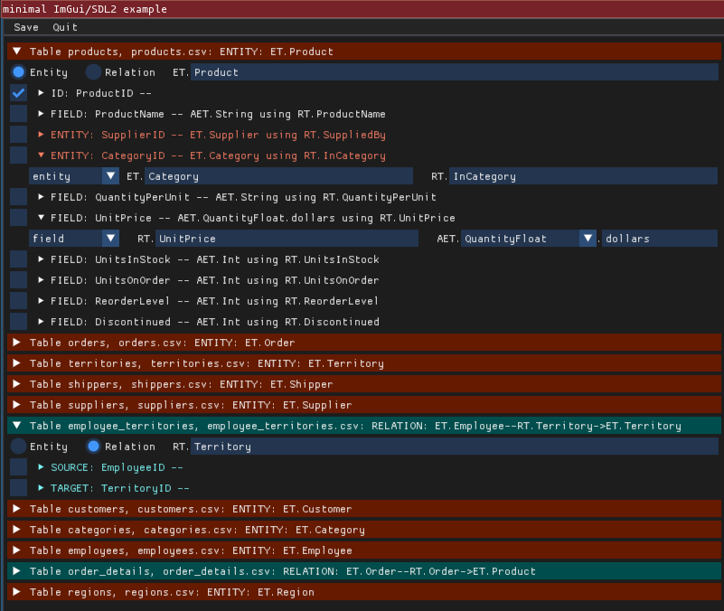
To get rid of the clunkiness, and also indulge myself to explore a new package, I decided to write a little UI using pyimgui to better edit the file. Try it out on my sample sql_import.yaml with:!!!

python -m zef.experimental.sql_ui.wizard sql_import.yaml

You should see something like:

The UI is in its early stages so might not work fully. It also requires installing the pyimgui module with sdl support (i.e. pip3 install pyimgui[sdl2] or the like). Weirdly this seems to have problems with python version 3.10 on macos... we will be looking into this.

To read more about using this GUI, check out our docs page on Multiple interlinked CSVs

"relation" kinds of tables

If there is a one-to-many or many-to-many relationship between two objects in a SQL database, then there are various ways to represent this. In the Northwind example, the "Order Details" table demonstrates this, as it allows each Order to contain multiple different products (the one-to-many relation), with particular (order,product)-specific prices, quantities and discounts.

OrderIDProductIDUnitPriceQuantityDiscount
102481114120.0
10248429.8100.0
102487234.850.0
102491418.690.0
...............

Hence we can think of this table as not being entity-centric but rather relation-centric. Any fields (e.g. the UnitPrice column) is information that should be attached to the relation between the order and the product. As Zef graphs we always have directed relations, so we need to also specify a "source" and "target" column:

OrderIDProductIDUnitPriceQuantityDiscount
PurposeSourceTargetFieldFieldField
ETET.OrderET.Product
RTRT.UnitPriceRT.QuantityRT.Discount
Data typeIntIntQuantityFloat.dollarsIntFloat

The import!

My full processing of the CSV files is shown below. My edits to the sql_import.yaml file are available here: sql_import.yaml.

from zef import *
from zef.ops import *
from zef.experimental import sql_import

decl = sql_import.guess_csvs("*.csv")
decl | write_file["sql_import.yaml"] | run

# ... edit sql_import.yaml externally...

decl = "sql_import.yaml" | load_file | run | get["content"] | collect
g = Graph()
actions = sql_import.import_actions(decl)
actions | transact[g] | run

After this import, the graph looks like:

>>> yo(g)

<...snip...>
^^^^^^^^^^^^^^^^^^^^^^^^^^^^^^^^^^^^^^^^^ Atomic Entities ^^^^^^^^^^^^^^^^^^^^^^^^^^^^^^^^^^^^^^^
[6007 total, 6007 alive] AET.String
[2985 total, 2985 alive] AET.Float
[2527 total, 2527 alive] AET.Int
[2232 total, 2232 alive] AET.QuantityFloat.dollars
[2469 total, 2469 alive] AET.Time

^^^^^^^^^^^^^^^^^^^^^^^^^^^^^^^^^^^^^^^^^^^^ Entities ^^^^^^^^^^^^^^^^^^^^^^^^^^^^^^^^^^^^^^^^^^^
[1660 total, 1660 alive] ET.Order
[154 total, 154 alive] ET.Product
[12 total, 12 alive] ET.Employee
[93 total, 93 alive] ET.Customer
[53 total, 53 alive] ET.Territory
[4 total, 4 alive] ET.Region
[3 total, 3 alive] ET.Shipper
[29 total, 29 alive] ET.Supplier
[8 total, 8 alive] ET.Category

^^^^^^^^^^^^^^^^^^^^^^^^^^^^^^^^^^^^^^^^^^^ Relations ^^^^^^^^^^^^^^^^^^^^^^^^^^^^^^^^^^^^^^^^^^
[4 total, 4 alive] RT.RegionDescription
[4 total, 4 alive] (ET.Region, RT.RegionDescription, AET.String)
[2155 total, 2155 alive] RT.Order
[2155 total, 2155 alive] (ET.Order, RT.Order, ET.Product)
[9 total, 9 alive] RT.ReportsTo
[9 total, 9 alive] (ET.Employee, RT.ReportsTo, ET.Employee)
<...snip...>

If you don't want to do the import yourself, you can also look at the graph that I created at the tag zef/blog/northwind, that is, you can access it via:

g = Graph("zef/blog/northwind")

Final comments

As always, answering a simple question has opened up many more questions which I can't help myself but discuss below...

One final purpose: "field_on"

There's another addition that's needed to import many production SQL tables: a way to handle databases with optimised tables.

While we do not need this kind of purpose for the Northwind dataset, it is useful to mention it to "complete the story". The above example of the "Order Details" table which produced pure relations (and not entities) is because the Northwind dataset is in "first normal form".

A "denormalised" dataset could also be used for performance reasons. For example, obtaining all of the products ordered by a particular customer would require an SQL JOIN query to obtain:

SELECT DISTINCT(order_details.ProductID)
FROM order_details INNER JOIN orders
ON order_details.OrderID = orders.OrderID
WHERE orders.CustomerID = "VINET";

Instead, the join of orders and order_details could itself be stored as a table (or view) in the SQL database:

OrderIDCustomerIDOrderDate...ProductIDQuantity...
10248VINET1996-07-04...1112...
10248VINET1996-07-04...4210...
10248VINET1996-07-04...725...
10249TOMSP1996-07-05...149...
10249TOMSP1996-07-05...5140...
.....................

The concept of avoiding joins is rather weird when coming from a graph perspective, as the equivalent of joins are trivial on a graph. However, you may not have any choice in the data you want to import. In this case, we can mark those columns as belonging to the relation between the order and product using "field_on":

OrderIDCustomerIDOrderDateProductIDQuantity
PurposeIDEntityFieldEntityfield_on
ETET.OrderET.CustomerProduct
RTIDCustomerRT.OrderDateRT.ProductRT.Quantity
TargetProductID
Data typeIntIntTimeIntInt

Here the "Quantity" column cannot be set as a field as it would have multiple values for the same ET.Order. So instead we designate that it should be attached to the "target" column ProductID. This means we could write a Zef query for the total quantity of an order as:

z_order > L[RT.Product] >> RT.Quantity | value | add | collect

Batteries-included?

The imported tables still duplicate a lot of information. For example, each of the ET.Order, ET.Supplier, ET.Customer, ET.Employee have a RT.Region which is a scalar string. This is not very connected, as it would be better to have these RT.Regions point at a ET.Region. That way, we could ask for all suppliers in the same region as a customer without doing string matching.

I was tempted to add this in as another purpose, something like entity_from_matching_field. But this would have degenerated into providing an arbitrary language to describe the endless possible databases out there. Instead, we can post-process the imported Zef graph, which gives us access to the entire Zef ops capabilities.

You might be worried about exposing the gorey details of the import process and only the post-processed data. This is easy, if we export only g | now to a new graph after performing the post-processing.

A comment on speed

If you run the commands in this blog post on a large dataset, then you are going to be waiting several minutes for the import. Even as part of writing this post up, and using the Northwind dataset which is relatively small, I found I had to optimise some aspects of the GraphDelta implementation.

This is largely due to the current pure-python implementation of the evaluation engine for ZefOps. In the future this will be implemented in C++ along with the core of the GraphDelta code.

Import directly from SQL

To be honest this blog post is a little crude, using CSV files which lack type information rather than the SQL source directly. The information available in the SQL schema can also assist automatic detection of connected entities and whether a table represents a single entity or many-to-many relations.

The benefit of handling CSV files is it allows us to accomplish almost all kinds of imports, so long as we provide enough additional information. If we supported only SQL, then this would limit the flexibility.

The other reason that the SQL schema is not used directly, is that it's a fair bit more work to support a SQL connection or export. But our intent is to extend these tools and make imports as close to one-click as possible!

Analysis using external tools

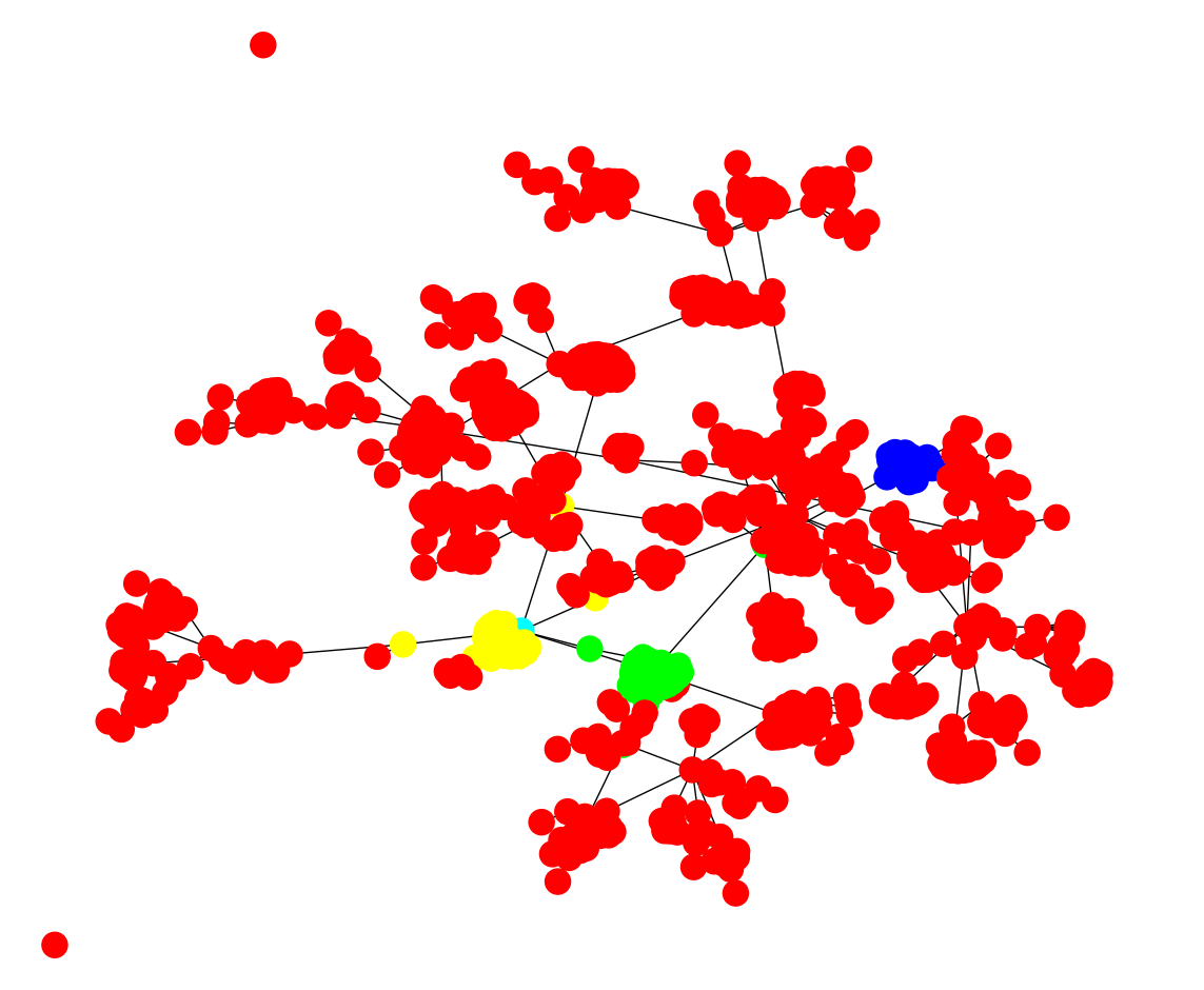
I'll leave this for the next blog post! But as a sneak preview...

Wrap up

If you'd like to find out more about Zef and ZefHub (and get early access), get us out at zefhub.io.

· 13 min read

One major motivating factor that is often associated with relational databases is the ability to interact and query the data declaratively. Instead of telling the DB exactly how to traverse and gather the data, just give a bunch of clauses that have to be true and let the DB figure out how to resolve the query most effectively.

q1 = Query([
Z['p1'] | is_a[ET.Person],
Z['p1'] >> RT.FirstName | value | equals['Roger'],
])
SELECT * from Persons WHERE FirstName="Roger"
  • everything in SQL is a table: entities are defined as rows of attributes. In Zef an Entity can "just be". It may have have attributes expressed as relations to values or atomic entities.
  • variables from predicate logic are the equivalent of columns / column names in SQL.
q2 = Query([
Z['x1'] | is_a[VT.Int],
Z['x1'] | less_than[5],
Z['x1'] | greater_than[0],
])
  • Z['x1'] is a variable in the sense of predicate logic. In other fields they are sometimes also referred to as "unbound constants".
  • We have to wrap it with Z, since using x1 by itself on the spot would not be valid Python syntax
  • We could declare all variables used beforehand if the Z bothers us: x1 = Z['x1']
  • each line is a predicate function: given a potential solution, it can be evaluated to true or false
  • these predicate functions are often called "clauses" in mathematical logic - don't be frightened by the name
  • each line can contain one or more variables: predicates can thus also express constraints between variables.
  • the solution to a given query / list of constraints MUST fulfill each individual predicate. I.e. it can just be seen as one big predicate function obtained by combining all of them via an And.
  • This combined predicate function is a function of all variables occurring in the query.
  • We can also see each individual predicate function as a function off all variables in the query if we want a more formal justification for combining them with an And (the logical operators can only combine predicates with the same function signature)

Let's take the previous query up a notch:

q3 = Query([
Z['p1'] | is_a[ET.Person],
Z['p2'] | is_a[ET.Person],
Z['p1'] >> RT.FirstName | value | length | equals[
Z['p2'] >> RT.FirstName | value | length
],
])

Just to put it in normal words: "please return me all pairs of persons whose first names are of the same length." A result of this query would be a (possbily very long) list of dicts, each containing two people [{'p1': z_jack, 'p2': z_john}, ... where z_john and z_jack are both ZefRefs and point to persons with those names respectively.

But this is not what we want to get at. The crucial part we want to demonstrate here is that to express queries of this type succinctly, we need the ability to use ZefOps inside predicate functions. It is crucial that these are not lazy values that can be evaluated to a fixed value beforehand, but they involve variables themselves. These only become equivalent to lazy values within the context of a potential solution.

So what is the problem? Before we were using greater_than[0], i.e. a value inside the combinator, whereas now we are using a clause. Also: clauses can be understood as Zef lambda functions (as we discuss elsewhere). And Zef lambda functions are values themselves within Zef: value semantics is one of the foundational principles that we cannot give up. So now we are using greater_than with two different values, but in quite different ways. This is a problem: what is the nature of the thing we pass into equals? Should the second case only return true if the argument piped in is the very Zef Lambda function inside? This seems to be the case at first glance, if we want strict and general value semantics. But there is a way out and one also encounters it in different contexts. It is actually an approach that dates all the way back to Alonso Church, who came up with lambda calculus, which you may have heard of. The way out of our dilemma is just to put on our Church glasses: in lambda calculus everything is a function. Even an integer like 42 can be seen as a function: it is simply the function that returns 42 whatever argument you give it. What are the arguments here and why are they not listed? Because it would be too tedious. As we saw, a query can be seen as one big lambda function itself that is just the combination of all listed clauses combined with And. The variables are implicit and are all the variables that occur in the query. This allows us to keep our short syntax in terms of values above, e.g. use greater_than[0] with it having exactly the simpler meaning we associated with it before. The occasional user of Zef does not even need to be aware of all this abstract stuff and lambda calculus.

So what does this mean concretely? How can we construct a semantically consistent system out of this? There is a very narrow path out of this mess. We can simply be guided by the logical constraint and the goal of a succinct, not overly technical syntax. We do not want to require everyone to have to syntactically wrap their values in a lambda function.

Let's go through the requirements:

  1. A value 42 is distinct from the Zef lamba function func[42] that always returns 42.
  2. values inserted into logic operators must be interpreted as Zef Lambdas
  3. We don't want to write the func[...] wrapper everywhere
  4. All of this is not specific to equals, but applies to all logic operators (unary, binary, all arities)

Hence, anything injected into a [...] of a logic operator will be understood to be wrapped by a func[...] at the point of evaluation. This may sound horribly complicated at first, but keep your pitch fork down for a moment. What we're after is that the resulting syntax is easy to use and consistent. The expression 42 | equals[42] will continue to evaluate to true, since the two associated Zef lambdas (which are values themselves) are considered to be equal.

Side note: note that lambdas in Python do NOT follow value semantics for functions in this sense:

my_answer_to_everything   = (lambda : 42) 
your_answer_to_everything = (lambda : 42)
should_we_start_a_flame_war: bool = my_answer_to_everything != your_answer_to_everything

# OMG Python, you're worse than social media!
print(should_we_start_a_flame_war) # True

But now we notice that this also allows us to throw in other expressions and operators that will be interpreted accordingly: both cases that we started off with, e.g. using greater_than[0] and but also greater_than[ Z['x1']>> RT.Age | value ] would work. At the point of evaluations, the latter internal argument is translated into func[ Z['x1']>> RT.Age | value ] which by itself is a valid Zef lambda function that could be used in a different context as well.

The one thing we are not allowed to do is wrap the expression in an additional func[] layer and expect the same behavior. E.g. equals[ func[Z['x1']>> RT.Age | value] ] would check whether the incoming value is equal to that lambda function, i.e. at the point of evaluation func[ func[Z['x1']>> RT.Age | value] ] is the Zef lambda function that always returns the internal lambda function (a value itself), not matter what arguments are passed in.

So what does this mean, you may ask? The take away message for Zef lambda syntax is that multiple layers of func[...] do not automatically collapse to a single wrapping func[...] layer. They are different things.

What about using Python lambdas in piped expressions? since 42 | (lambda x: x+1) cannot be intercepted by Zef in any way without doing unspeakably horrible things, you will have to wrap raw python functions and lambdas in one layer of func[...]:

42 | func[lambda x: x+1] | collect

works and is the way you have to do it. The same goes for normal python functions. But as soon as you have a Zef function, wrapping it in a func[...] will cause an additional layer of wrapping, since that Zef function is itself already a Zef value. This is the gotcha to watch out for!

SQL & Zef

Declarativeness is in the Eye of the Beholder

Knowing ones own type

How does an entity / object know what it is?

Classes / Structs

This depends on the programming language. In dynamic languages like Python, this is stored as explicit meta-information as a pointer on each object pointing at the parent type object. In compiled languages like C++, this information may not even be stored explicitly at runtime: only the struct's/object's contained attributes are stored at the objects location in memory. The information about which type it is compiled away in the simple case (this may be different for typed unions, e.g. std::variant and other more advanced structures).

JSON / Python Dicts

This is either implicit from the context in which the dictionary is stored. Often the associated entity's type may also be explicitly stored as a value under a "type" key.

Relational Databases / Spreadsheets

Which table it is contained in: the table name can often be seen as the equivalent to the object's type. Each row in the table can be seen as an object/entity expressed in terms of its attributes / fields (columns).

Document Database

These are often organized in terms of collections. Just like we know that the real world entity described by a row in a table knows what it is from the table's name, a document in a collection is specified by the name of the collection. In some cases users may find it more convenient to directly dump json into the database.

Zef Graphs

Each Relation / Entity / Atomic Entity (RAE) has its type stored explicitly in its blob on the graph. In contrast to objects, RAEs have no internal structure whatsoever. Rather than choosing to model the world in terms of a hierarchical taxonomy, all information is represented associatively in terms of relations.

History of Zef: Evolving from Property Graphs

"Perfection is achieved, not when there is nothing more to add, but when there is nothing left to take away." — Antoine de Saint-Exupéry

The Zef data model may seem somewhat strange at first when coming from the world of objects, tables or property graphs. In this post we want to give a brief overview of how we arrived at this data structure. Maybe we can even convince you that it is a simpler data structure than many of the better known alternatives.

1) model our domain in terms of C++ structs / Python objects 2) move to using plain old dictionaries, all the serialization and de-serialization code was getting too much 3) having to choose a hierarchy does not play well with modelling a complex domain where requirements often change. We often thought we got the domain modeling wrong, but that was missing the true underlying reason: the real world domain model was that of a graph and different parts of our system require querying the data from different directions. Choosing any tree-based hierarchical data structure has a structural mismatch with the true domain model. We moved on to use NetworkX. What a relief, working directly in terms of graphs is awesome! Why is this not the norm? 4) NetworkX is a bit slow. Even for Python standards. Also, we really want to work on top of graphs in our high performance simulations written in C++. 5) After exploring multiple options (iGraph, Boost Graph, various DBs), we didn't find any that had user friendliness in terms of the API we were looking for and the performance we required. How hard could it be to build a more performant version, but very much stripped down version of NetworkX in C++ and expose bindings to Python. This was actually easer than we thought and a basic version of "Arachne" was up and running after two to three weeks. The core data structure was a directed property graph: both the nodes and edges could contain attributes. For the application that we were running (MCTS-like simulations), Arachne achieved about a 10000x speedup over NetworkX, which somewhat surpassed our expectations. Cache locality and data oriented design for the win! 6) This design took us pretty far, but there were three problems appearing. A) working in the field of manufacturing, our domain models between customers differed and were often quite complicated. Also, they were often evolving over time as new requirements and features came up. We noticed the following pattern reappear every few weeks: an initially unimportant field of some entity started off its life as an internal attribute on a node or an edge. But at some later point, it became more important and modelling it as an internal attribute no longer seemed like the right choice. It should be a separate entity on the graph. All of this implied a graph schema change (yes, Arachne graphs had schemas) and a migration of the production data together with all the different code snippets that tied into that attribute. We also noticed that the opposite direction never occurred: something we had started modeling as a separate entity on the graph never became an internal attribute and caused us hours of repetitive, boring work.

With this pattern emerging, what would the end game of this iterative domain model revision war be? A domain model where every attribute will have become its own distinct entity on the graph? That sounds silly and too radical. But what would happen if we actually tried this? What is the defining difference between an objects attribute and a separate entity connected by a relation in any case? Doesn't this distinction introduce two different languages for querying individual fields of entities on a graph: one for traversing the graph and one for accessing internal attributes. Would it not be simpler if we had a single language only and everything would just be a graph traversal. There is no inner structure to RAE, there is no externally imposed hierarchy on our domain model.

There was one complication though: Since Arachne was a directed property graph, we stored attributes for some relations on the graph as well. It was by far not as common as attributes of an entity, but they were extremely useful in some cases (suppose you were to model an online store with certain items added to an order. One of the simplest ways to store the number/amount of a given item is as an attribute of the "ordered" relation itself). What would become of these edge attributes when we flatten everything out on the graph? According to our recipe of representing fields as relations to separate "values nodes" on the graph, we would have relations coming out of relations?! This would no longer be a graph. However, after a fair amount of back and forth, this is exactly what we decided to do. Zef Graphs are thus not simple graphs, but "meta-graphs" (we found this naming in this paper by Ben Goertzel). Note that these are different from hypergraphs, which can have edges which can connect more than two nodes.

· 6 min read

In the last blog post, we created a console-playable Wordle game in few lines of Python using ZefOps. In this blog post, we will write a Wordle solver (or more like your own Wordle assistant) that suggests what your next move could be 😎

So before digging deeper, be sure to check part 1!

Wordle

What will we do? 🤔

Our aim by the end of this blog post is to write a solver that given a list of guesses + discarded letters = a list of possible answers. So you can think of it as an eliminator of bad guesses given our previous guesses.

The idea is pretty straightforward, and given our first one or two guesses are good enough, we can arrive at the correct guess in around 4 guesses 😲 wordlist Let's look at an example:

["a", "b", "3", "c", "5"] | filter[is_alpha] | collect      # returns ["a", "b", "c"]

Each item of the list passes through the filter's predicate which evaluates to a boolean value True or False. If the value is True the item passes the filter, otherwise it gets discarded.

PS: is_alpha is a ZefOp that takes a string and checks if its is only consists of english alphabet and then returns True or False

So if we pass the wordlist through enough filters we will reduce our wordlist to only the possible guesses at that stage. So the more information we have, i.e correctly placed letters or misplaced letters, the more filters we can create.

Let's start building 🏗

  • Start by importing ZefOps and loading our word list
from zef import * 
from zef.ops import *

url = "https://raw.githubusercontent.com/charlesreid1/five-letter-words/master/sgb-words.txt"
wordlist = url | make_request | run | get['response_text'] | split['\n'] | map[to_upper_case] | collect
  • Let's add our discarded letters and guesses from the game we are stuck on
discard_letters = 'ACLNRT'

guesses = [
["_", "_", "_","_","[E]"],
["_", "U", "_", "[E]","S"]
]
  • Now let's write our filters generator ⚙️
def not_contained_filters(discard_letters: str):
return discard_letters | map[lambda c: filter[Not[contains[c]]]] | collect

def correct_or_misplaced_filters(guess: str):
misplaced = lambda p: [filter[Not[nth[p[0]] | equals[p[1][1]]]], filter[contains[p[1][1]]]]
correct = lambda p: [filter[nth[p[0]] | equals[p[1]]]]
return (guess
| enumerate
| filter[Not[second | equals['_']]]
| map[if_then_else_apply[second | is_alpha][correct][misplaced]]
| concat
| collect
)

Believe it or not, this is all we need. It might look complicated but it is simpler than it looks. So let's dissect it 🗡

Basically, these 2 functions use ZefOps to generate ZefOps of type filter with baked-in predicate functions given both the discarded_letters and our previous guess.

Function: not_contained_filters

Let's look at the first function not_contained_filters. The function takes the discarded_letters as a string and maps each letter c to a filter function that has a predicate function Not[contains[c]]] which is the ZefOp Not taking as an argument another ZefOp contain.

If this looks complex try to read it as an english sentence. filter what doesnot contain the letter c So given this example ["ZEFOP", "SMART"] | filter[Not[contains["A"]]] | collect only ZEFOP will pass the filter.

Do you wanna guess the output when we pass discard_letters = 'ACLNRT' to this function as an argument?

Well, we are mapping each letter of that string to a filter so we end up with this OUTPUT:

[
filter[Not[contains['A']]],
filter[Not[contains['C']]],
filter[Not[contains['L']]],
filter[Not[contains['N']]],
filter[Not[contains['R']]],
filter[Not[contains['T']]]
]

A list of filters one for each discard letter. This way any word that doesn't pass all these filters will not be part of our possible answers.

Function: correct_or_misplaced_filters

Let's look at the second function 'correct_or_misplaced_filters', which is pretty similar to the one above. We are returning filters for when we have a correctly placed letter or a misplaced letter. This function could be divided into 2 other functions, but with the if_then_else_apply ZefOp we can simply do it in the same function without duplicating the logic. The apply at the end of of the ZefOp name means we apply the passed functions to the first argument.

Let's take a closer look at the return statement of this function and run our second guess from our guesses list above to walk through the function logic:

OUTPUT:

misplaced = lambda p: [filter[Not[nth[p[0]] | equals[p[1][1]]]], filter[contains[p[1][1]]]]
correct = lambda p: [filter[nth[p[0]] | equals[p[1]]]]

guess = ["_", "U", "_", "[E]","S"]
(guess # ["_", "U", "_", "[E]", "S"]
| enumerate # [(0, "_"), (1, "U"), (2...]
| filter[Not[second | equals['_']]] # [(1, "U"), (3, "[E]"), (4, "S")]
| map[if_then_else_apply[second | is_alpha][correct][misplaced]] # [[filter[nth[p[0]] | equals[p[1]..]
| concat # [filter, filter, filter..]
| collect
)

The comments show the transformation the guess input is going through until we get out a list of filters that contain predicate functions that satisfy correct and misplaced letters requirements.

So the output of this snippet given the guess = ["_", "U", "_", "[E]", "S"] is this OUTPUT:

[
filter[nth[1] | equals['U']], # Second letter should equal U
filter[Not[nth[3] | equals['E']]], # Fourth letter should NOT equal E
filter[contains['E']], # Word contains an E
filter[nth[4] | equals['S']] # Fourth letter should equal S
]

Put it all together 🧩

When we put both of these functions along with our 2 inputs we end up with a pipeline of filters that we can run the whole wordlist through.

filters_pipeline = [
filter[length | equals[5]], # Just making sure it is a 5 letter word
not_contained_filters(discard_letters),
guesses | map[correct_or_misplaced_filters] | concat | collect
] | concat | as_pipeline | collect # Flatten all sublists and turn them into a pipeline

We are creating a list of filters coming from the discarded letters and the mapping of each guess in our guesses.

PS: as_pipeline takes a list of ZefOps and returns a single ZefOp that we can call or pipe things through

possible_solutions = wordlist | filters_pipeline | collect
possible_solutions | run[print]

We pipe our entire wordlist through the filters pipeline to end up with all possible solutions. In this example, given our wordlist and guesses+discarded letters the possible solutions are: ["GUESS"], who could have guessed that 😉

Wrap up 🔚

And just like that we used ZefOps to generate ZefOps that are used with other ZefOps on our wordlist.. Pheww, how Zef!

Given this code is pure ZefOps and ZefOps compose, we can reduce it into one line. But let's not do that, or may be...

Worduel 👀

In part 3 of this series, we are going to take this to the next level, where we will use ZefDB, ZefGQL, ZefFX to create a competitive web game of Wordle where you can take your friends, collegues, or your mom to a game of Worduel 😜

· 8 min read

In this blog post we are going to build a console-playable Wordle game using Python and zef in 30 lines 🔥

The purpose of this blog is to showcase the usage of ZefOps to create easy, readable, composable, extendable, highly-decoupled, and [enter more buzz words here 😍] code!

So before getting started, let's quickly review what is Wordle?

Wordle

What is Wordle? 🤔

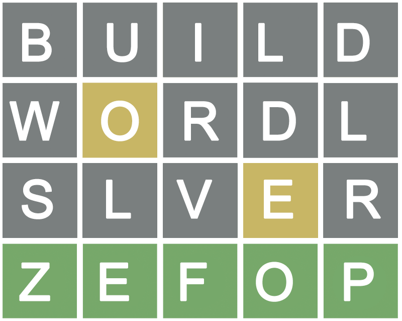
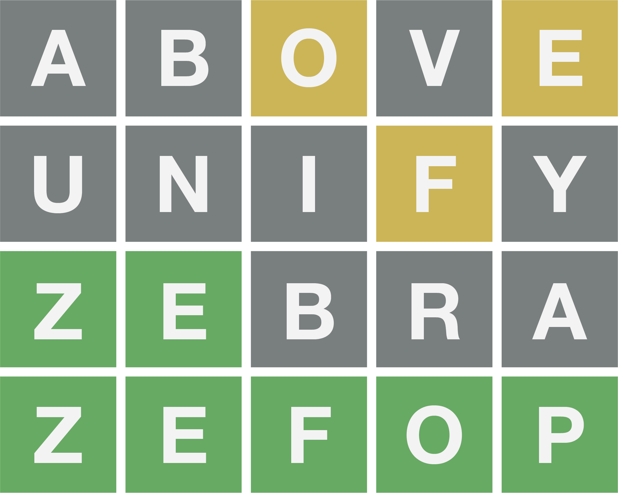
Wordle is a simple game where you have six chances at guessing a five-letter word.

After each guess, the game will give you hints.

  1. A green tile means that you guessed the correct placement of a letter.

  2. A yellow tile means that the letter is in the word, but your guess had the wrong position.

  3. And lastly, a grey tile means the letter is not in the word.

Rules 🔢

So the rules are pretty straightforward. Given we are playing the game in a console, let us remap the rules a bit.

After each guess,

  1. A letter appearing by itself == Green tile 🟩

  2. A letter appearing with [ ] around it == Yellow tile 🟨

  3. A dash appearing means == Grey tile ◻️

Building the game 👷🏻

To run the code below, you'll need early access to Zef (it's free) - sign up here!

  • Let's import ZefOps. Any operator we might need should be there 😜
from zef import * 
from zef.ops import *
  • Then we load our 5-letter word list

For this example I am using this wordlist I found on Github.

Using ZefOps, we can either load the list from a link, a file stored locally, or simply from your clipboard 😲

# Load from request response (Choose this one)
url = "https://raw.githubusercontent.com/charlesreid1/five-letter-words/master/sgb-words.txt"
wordlist = url | make_request | run | get['response_text'] | split['\n'] | map[to_upper_case] | collect

# Load from local file
wordlist = 'wordlist.txt' | load_file | run | get['content'] | split['\n'] | map[to_upper_case] | collect

# Load from clipboard
wordlist = from_clipboard() | run | get['value'] | split['\n'] | map[to_upper_case] | collect

We can already see the power and ease of ZefOps. In just one line we are able to load a string of words, split it on new lines, then convert each string to uppercase.

We will get more familiar with the lazy nature of ZefOps and why we need "collect" in a bit. But notice, to go from one stage to another aka transform your input, you just have to pipe | operators. This way your input will flow through your operator chain aka pipeline giving you the output you need.

  • Now we initialize some game related variables
# Game Variables
counter, to_be_guessed = 6, random_pick(wordlist)
discard_words, discard_letters, guesses_list = set(), set(), []

Btw, random_pick is also a ZefOp. Given a list, a string, or a simple iterable, it returns a random item/character from the input. So here, given our words list, we choose a random word that we will have to guess.

Also notice we can call ZefOps similar to a function using zefop(args).

  • Now for some ZefOp 🪄 magic 🪄
# Predicate function constructed using zefops
is_eligible_guess = And[length | equals[5]][contained_in[wordlist]][Not[contained_in[discard_words]]]

Using ZefOps, we're able to pack a lot into a single line (and still maintain readability). Let's look into it:

  1. Firstly, this ZefOp declares a function that takes an input string and checks if its length is equal to 5 and is contained in the word list and it is not a previous guess.

  2. If you pay attention we didn't have to pass an input yet or even compute a result. You can think of this as a mini program, one that we can use in multiple places, and extend easily by piping more ops into it. We've also just designed our very own ZefOp composed of other ZefOps. The beauty of it all it is just data 0️⃣1️⃣ more on that later...

  3. "CRANE" | is_eligible_guess turns into a LazyValue. Put simply, a value + zefop is a LazyValue 🥱. A LazyValue is not computed until we do | collect to make it eagerly execute. We will see more value out of LazyValues later on.

  • Now for the meatiest 🥩🥩🥩 part of the code
def make_guess(guess, to_be_guessed, discard_letters):
def dispatch_letter(arg):
i, c = arg
nonlocal to_be_guessed
if c == to_be_guessed[i]: # Rule 1 🟩
to_be_guessed = replace_at(to_be_guessed, i, c.lower())
return f" {c} "
elif c in to_be_guessed: # Rule 2 🟨
to_be_guessed = replace_at(to_be_guessed, to_be_guessed.rindex(c), c.lower())
return f"[{c}]"
else: # Rule 3 ◻️
if Not[contains[c.lower()]](to_be_guessed): discard_letters.add(c)
return " _ "

return (guess # "CRANE"
| enumerate # ((0, "C"), (1, "R"), ...)
| map[dispatch_letter] # ["_", "[R]", "_", ...]
| join # " _ [E] _ _ _ "
| collect
), discard_letters

This is the main logic behind Wordle. After each guess, we match our guess characters with the actual word. The focus of this function is in the return statement of the function. It is a chain of ZefOps that takes our "guess" as an input.

We run our guess word through enumerate to get back a list of tuples of (character, index). We then pass that list to map, which is a ZefOp that, as the name suggests, maps each item of an input to an output given a dispatch function which we pass as the second argument using [ ]. The output of map is always a list of the individual outputs, so we pipe through | join to connect the list as a string. collect is finally piped so we evaluate this LazyValue.

discard_letters isn't part of the game logic but just makes it more playable.

Psst: join can be called with a joiner i.e join["_"] instead of the default which is empty string join[""]

Polishing and running ✨

Now we have to use these 2 simple functions along with couple of ifs and some more ZefOp 🪄 magic 🪄 to make the game playable!

"~Welcome to Wordle~" | run[print]    # boujee way of printing using zefops

while counter > 0:
guess = input("Your guess:").upper()
if is_eligible_guess(guess): # Calling our predicate zefop on the guess
counter -= 1
discard_words.add(guess)
guess_result, discard_letters = make_guess(guess, to_be_guessed, discard_letters)
discard_string = discard_letters | func[list] | sort | join | prepend [' [Not in word]: '] | collect
guess_string = guess_result | pad_right[20] | append[guess + discard_string] | collect
guesses_list = guesses_list | append[guess_string] | collect
guesses_list | join['\n'] | run[print]

if guess == to_be_guessed:
f"Your guess {guess} is correct!" | run[print]
counter = -1
else:
f"{'Previous guess' if guess in discard_words else f'Invalid guess {guess}'}! Try again." | run[print]

if counter == 0: f"Your ran out of trials, the word was {to_be_guessed}" | run[print]
  • Okay, so what's going on?

"While" allows you to loop until a condi... I am joking 🤡 I know you are looking at those lines with zefops.

  1. discard_string is a string of all the letters we guessed over time that aren't part of the word we are trying to guess. We compute it by taking the set of discard_letters piping it through func[list] which is equivalent to casting set to list. Then we sort it and join it into a string. Finally we prepend another string to the string we created. prepend/append work on both list and string.

  2. guess_string is the guess_result piped through pad_right which pads our string with whitespace to a specifc length. Then we append our guess and discard_string to the padded string.

  3. guesses_list is appended with the guess_string. This is just to print out the full list of guesses nicely in the console after each guess.

  4. join appears again but this time with the new line joiner. We pipe through run[print] to perform a side effect of printing to the console. collect is used when computing a result.

Wrap up 🔚

Just like that, in 30 lines (or less) we created Wordle in Python using ZefOps!

The takeaway from this is how easy ZefOps are. They are short. They are composable. They are lazy. They are data. They are extensible. They are pure. They are Zef!

If you'd like to find out more about Zef and get early access to run this code yourself, sign up on zefhub.io. It's completely free, we won't bombard you with emails, and we'll get you set up quick!

Stuck? 😰

If you are stuck and want some help, in part 2 we create a Wordle solver using Python and ZefOps.